LLMs: Understanding Tokens and Embeddings
The Background Story
Enabling Computers to Read
It’s well understood that machine learning systems do not deal with text directly. Or for that matter, images, audio and video.
For text, we first convert them to numbers by some mechanism before we feed them into our machine learning systems.
The strategies for converting into numbers exist in various forms. And choosing one over the other depends entirely on the architecture of the consuming system.
Until the deep-learning approaches to working with text came onto the scene, we mostly dealt with words and converted words into numeric identifiers. Words are a group of characters delimited by spaces and punctuations. Something we are all familiar with. As we will see further, it’s not necessary that we segment text only at spaces and punctuations. We can even break down a single word into many units - these units are what we call as tokens.
Tokens are the fundamental unit we deal with as one of the outcomes of the text preprocessing, and they are further mapped to numeric identifiers. Each token maps to a unique numeric identifier.
Once the identifiers are associated with a token, dealing with them is as good as dealing with their associated tokens. Any statistical processing over tokens (like, their counts, or co-occurences) can be done by dealing with their associated identifiers.
Words are natural candidates for processing as tokens because they are first-class elements of our natural language. But tokens are more general - a single word represented as consisting of multiple tokens is perfectly normal. And a token can even span multiple words, not necessarily starting and ending at word boundaries. (This - the latter part - may not make complete sense just yet.)
We store the words to ids relationships in a table. Within the context of a given system, we are required to be consistent in using this mapping table throughout.
But, Problems…
Unlike the ideal world, the real world can throw a lot of surprises. Let’s say, we use the identifier 1048 for the word dog.
But, dog at the beginning of a sentence will appear as Dog. Are they the same words?
Also, consider the possibility of mistyping by a human wherein the word was typed as DOg. We humans will be able to process it, but the computer is unlikely to be able to deal with it. Unless, we treat all words in a case-insensitive manner by down/up-casing everything.
That’s great, you say, but what about Dawg? Oh, well. That’s a spelling mistake and we can’t handle it.
| token | id |
|---|---|
| dog | 1048 |
| Dog | ?? |
| DOg | ?? |
| Dawg | ?? |
Then, there are other problems too. What about words that don’t exist in our dictionary? If we haven’t seen a word, we’d have no identifiers for it. Dawg is only one example, and it is a possible speeleeng myshtake. But new words get introduced into a language all the time.
Dealing with the Problems
What if we process text by breaking it down into characters!?
So, how about splitting Dawg into four tokens - D, a, w, g.
We thus convert all text into character-level tokens and then, deal with their numeric identifiers.
Sounds insane, and maybe it is! Until, we throw huge amounts of compute power at our problem. Given a very very large scale processing infrastructure, we can indeed compute language level statistics to such level of detail that we might be able to re-construct a language from statistical priors of just the characters!
Don’t believe? Go check Andrej Karpathy’s demonstrating how to do this from scratch here.
LLMs compute the probabilities of long sequences of characters. During training, they compute and remember the distribution from the training data. During generation, they predict - based on what they have learnt. Conceptually, it’s that simple!
Assume a sequence length of 100 characters, and 26 characters, assuming lower-case alphabets without numbers. That makes \(26^{100}\) possible combinations - surely, an oversimplification. And sure enough, all characters are not independently random. So, given enough training data, there is a great chance that a large enough computer can calculate prior probabilities and then use those to predict next character tokens when we input a new piece of text from the same distribution.
In reality, we do wish to optimize here. On the one hand, working with character tokens is very inefficient. On the other hand, working with entire words - those space separated molecules of characters - troubles us with two problems
- A very large dictionary covering the entire natural language
- An inability to deal with words never seen before - either new words or spelling mistakes.
This leads us to another idea - processing input text into variable-length tokens using techniques like byte pair encoding (BPE). This technique does not tokenize at the natural word boundaries (like the space characters), and includes individual characters to sub-words and larger groups to be considered as tokens. This gives us flexibility, and a decent way to address the problems mentioned above.
Technically, you can encode larger chunks without ever stopping - but the key thing is that if there are very few instances of a “token” then it is statistical noise. The value is in seeing many of them and in some context to associate prior probabilities to them. This is also a key engineering knob - deciding where to stop when it comes to the vocabulary size.
Too small a dictionary means we have to calculate conditional probabilities over much longer sequences as the information gain over a shorter sequence is likely to be much lower. A very large dictionary might mean quite a few tokens will have no useful conditional probabilities that can be calculated with confidence.
Allowing characters and subwords to exist in the dictionary, along with some of the common whole words, and up to a limit that can be handled by the size of the model and the resources we are willing to commit to (memory, CPU) - should work well.
We’ll go into tokenization next, but before that, a few items of note.
Quick Supporting Glossary
- Python
- Needs no explanation. Most of ML you do these days are accessible easily through Python
- Numpy
- A vast Python library for numerical processing. ML is nothing if not numerical processing
- Huggingface
- A company, a community, to discover and share models, data, information. Maybe, the Github of the ML world!? Most open models and datasets can be found here, including those that common folks like us can publish. Loosely, the Docker Hub equivalent for ML.
- Transformers: In the context of Huggingface, a library they have published for generally dealing with the various models published on the hub.
- Model Card
- A card detailing important information of models. Example - the Llama 3 model card.
- Data Card
- Likewise, for published datasets.
When we refer to a model using an <org-id/model-name> convention - example, mistralai/Mistral-7B-v0.1. This points to the organization mistralai’s Mistral 7B v0.1 model repository on Huggingface.
Models are generally very large in size, and you do not want to download them again. More often than not, libraries aware of Huggingface manage downloading (and caching) model files from Huggingface and it’s only the first time you access a model do you see output on your screens showing transfers in progress. The second time onwards, locally cached data is used. Cached files are typically under $HOME/.cache/huggingface.
If you’d like to manage your own downloads and caching, you can use the official Huggingface tools like
While the model data will be automatically downloaded when you run the code, you can download them ahead of time using huggingface-cli, as shown in an example below.
huggingface-cli download meta-llama/Meta-Llama-3-8B
Finally, for getting the code used in this article, you’ll find links to download them at the end of this article. The variable names should be self-explanatory. Refer to the linked code towards the end for more details, including the various import statements.
And a Few Steps
To work with the code, you need to take care of a few things
- Install Python
- Install Poetry
- Optional, but strongly recommended - a virtual Python environment manager like virtualenv.
- Download the pyproject.toml file into a directory
- [Optional] Create and activate a virtual environment for Python
- Run `poetry update` within that directory
- Keep all python code within this directory
- Create an account on Huggingface.
- Run `huggingface-cli login` and follow instructions
- On Huggingface, visit the mistralai/Mistral-7B-v0.1 and meta-llama/Meta-Llama-3-8B pages and register/sign agreement to use those models.
Tokenization
Let’s jump into tokenization.
Tokenization creates a vocabulary or a dictionary for encoding the input text for further processing. Our choice ranges between using individual characters to using word tokens. Even beyond (length-wise), actually, but that doesn’t make much sense.
Tokenization is an important tunable part of the entire process. Tokenization choices will deeply impact the sizes of the network, the training effort, and the quality of the outcomes.
- Character-level tokens will keep your dictionary small. Word-level tokens will bloat your dictionary.
- With character tokens, you lose larger structures and patterns. With word tokens, you capture more of them
- Again, with character tokens, you are able to deal with every input never seen before. With word tokens, you will not be able to handle tokens/inputs never seen before.
The smart folks in this area have devised ways to keep the best of both worlds. Conceptually in a manner similar to Huffman encoding - the famous technique for compression - tokenization of input text is done, using variable-length chunks of text based on their frequencies as tokens. Thus, we have tokens that range from individual characters to those that can be complete words, and everything in between. This takes care of handling out-of-vocabulary words, while also capturing word-formation structures with the longer tokens. And since we use the longest-match, the size of the vocabulary does not affect the correctness of the tokenization activity. Better yet, you can choose the size of the vocabulary depending on your resource estimates.
It’s also interesting to note that with more tokens, we capture further structures of the language - how characters combine to form larger and larger structures. These can indirectly encapsulate patterns that represent notions like grammar, or how words form. These enable the downstream network to even deal with new words not seen before, and even misspellings!
Exploring Tokenization in Code
Let’s look at how mistralai/Mistral-7B-v0.1 does tokenization.
We use the transformers library from Huggingface. It has some pretty nifty utilities for working with a variety of models with literally no configuration steps. In particular, we will be using the two Auto* classes
The model data contains everything - metadata, token vocabulary, architecture, layers information, and more. So, using the Huggingface coordinates as strings (e.g., mistralai/Mistral-7B-v0.1) while invoking class methods on these above classes is enough - the transformers library pretty much does eveything else for the most common use-cases we are interested in.
On my machine, the model directory has the following files
-rw-r--r--  1 jaju  staff         596 Apr  8 10:43 config.json
-rw-r--r--  1 jaju  staff         111 Apr  8 10:43 generation_config.json
-rw-r--r--  1 jaju  staff  4943162336 Apr  8 10:52 model-00001-of-00003.safetensors
-rw-r--r--  1 jaju  staff  4999819336 Apr  8 10:49 model-00002-of-00003.safetensors
-rw-r--r--  1 jaju  staff  4540516344 Apr  8 10:51 model-00003-of-00003.safetensors
-rw-r--r--  1 jaju  staff       25125 Apr  8 10:43 model.safetensors.index.json
-rw-r--r--  1 jaju  staff       23950 Apr  8 10:43 pytorch_model.bin.index.json
-rw-r--r--  1 jaju  staff          72 Apr  8 10:43 special_tokens_map.json
-rw-r--r--  1 jaju  staff     1795303 Apr  8 10:43 tokenizer.json
-rw-r--r--  1 jaju  staff      493443 Apr  8 10:43 tokenizer.model
-rw-r--r--  1 jaju  staff        1460 Apr  8 10:43 tokenizer_config.json
You can inspect the tokenizer.json file for more insights. In fact, there are other plain-text JSON files too and I’d recommend scanning them.
Let’s pass some sentences to the tokenizer and see how it is broken into tokens. The transformers library gives you a pretty nifty API to deal with this processing, as you can see below. The tokenizer object is a function object.
tokenizer = AutoTokenizer.from_pretrained(mistral_model_name)

print(f"The vocabulary size is {len(tokenizer)}")

inputs = tokenizer("Who is Pani Puri?", return_tensors="pt")
input_ids = inputs["input_ids"]
print_tokens(tokenizer, input_ids)

inputs = tokenizer("Who is Katy Perry?", return_tensors="pt")
input_ids = inputs["input_ids"]
print_tokens(tokenizer, input_ids)
The vocabulary size is 32000
==============================
     Tokens and their IDs
==============================
Token      | ID
-----------+------------------
           | 1
Who        | 6526
is         | 349
P          | 367
ani        | 4499
P          | 367
uri        | 6395
?          | 28804
==============================
==============================
     Tokens and their IDs
==============================
Token      | ID
-----------+------------------
           | 1
Who        | 6526
is         | 349
Kat        | 14294
y          | 28724
Perry      | 24150
?          | 28804
==============================
Look at the tokens closely. Familiar word-level tokens are only incidental - depending on how Mistral chose the size of the vocabulary and the strategy, the tokens have been generated. You can observe the token vocabulary size - it’s a round number. And that was a choice made ahead of time. Also note the first token is empty space with id 1 - the tokenization strategy decides how (and if) to encode markers like a sentence/content start. The next model does it differently, as you’ll see.
Let’s run the above with the meta-llama/Meta-Llama-3-8B as well, for a comparison. What differences do you notice?
tokenizer = AutoTokenizer.from_pretrained(llama3_model_name)

print(f"The vocabulary size is {len(tokenizer)}")

inputs = tokenizer("Who is Pani Puri?", return_tensors="pt")
input_ids = inputs["input_ids"]
print_tokens(tokenizer, input_ids)

inputs = tokenizer("Who is Katy Perry?", return_tensors="pt")
input_ids = inputs["input_ids"]
print_tokens(tokenizer, input_ids)
Special tokens have been added in the vocabulary, make sure the associated word embeddings are fine-tuned or trained.
The vocabulary size is 128256
==============================
     Tokens and their IDs
==============================
Token      | ID
-----------+------------------
Who        | 15546
 is        | 374
 P         | 393
ani        | 5676
 P         | 393
uri        | 6198
?          | 30
==============================
==============================
     Tokens and their IDs
==============================
Token      | ID
-----------+------------------
Who        | 15546
 is        | 374
 Katy      | 73227
 Perry     | 31421
?          | 30
==============================
The tokens are different. But Llama 3, given that it has a higher token vocabulary size - about 4 times - and encodes with less tokens the sentence with words it has possibly seen before. But both tokenizers handle the possibly new words “Pani Puri” without a problem.
Also note that each token that covers a beginning of a word has a leading space. These minor-looking choices impact how the network looks at data and what it learns very significantly.
With a larger vocabulary, you can encode more in less. There’s more signal for less number of tokens.
Embeddings
Embeddings are an interesting next level to get to.
Tokens are only a preprocessing step. There are too many of them. If we wish to work with tokens, our neural network will probably need as many neurons in the input layer to process them. The simplest manner in which you can encode these tokens are via one-hot encoding. That makes for very sparse vectors, and very inefficient utilization of the many neurons at your service, given all except one would be idle when a token is ingested.
Consider the sentence - “I love my pet” - and this is our entire dataset.
| Token | Id |
|---|---|
| I | 1 |
| love | 2 |
| my | 3 |
| pet | 4 |
The sentence will be encoded into four vectors
[[1,0,0,0],[0,1,0,0],[0,0,1,0],[0,0,0,1]]
If our dataset was larger and had more tokens, the above vectors would be longer still with the additional elements all set to zero.
While we can certainly feed these one-hot token vectors as “features” to the neural network, they are very sparse and learning signals from them would be computationally very expensive - both in the processing cycles as well as memory. We probably can do better by converting them into a representation that captures better semantic relationships between them.
The denser the information content, the more you will be able to get from any machine learning effort, for the same architecture. While we make this statement very loosely, any claims of better semantic representations need to be validated thoroughly.
A Brief Build-up
This section steps into the generative LLM domain superficially, to make a case for embeddings. Please treat this section accordingly - as some background, rather than the depth.
For the moment, ignore the fact that tokens can be characters or just paired up bytes that don’t mean a thing in our natural language.
With an extremely large dataset - our text corpus - that is made up of long sequences of such tokens, we hope to still find enough patterns.
I’d encourage you to read the previous sentence once more, because I don’t know how to express it better but it’s profound yet very meh in how it comes out.
Humans can learn to speak without learning to read and write. They learn by hearing. When they hear, they have no notion of words and their boundaries. They have no notion of spellings, or the alphabet. We learn because we’ve heard for a very long time. Kids say their first words after being spoken to for very long. Even then, they start very unskilled and take a very long time before they can form complete sentences. But all along, they are still learning because the world does not stop talking to them. We are wired to decipher patterns and learn them. And then apply them.
Machines are the same - because they are based on our current best understanding of how the human neural network - the brain - works.
If we mimic the same processes by which humans learn, we might be able to make the machines work too. It’s funny I say that in a prophetic way because I don’t need to back myself up. The brave, smart folks in the past already hypothesized thus, and as of now (the year 2024), they have also proved themselves right. We’re only reading an article describing the current world - so, let’s move on.
Imagine a generalized problem where given a set of tokens occuring together in a sequence, we’d like to train a network that can predict the next token. Remember that we are talking tokens - not words. Also, remember that words can be tokens, but tokens need not be words.
Given a corpus of text, and tokens that form the vocabulary of that text, by training a neural network that can predict the next token well, we get a network that intrinsically captures relationships between them.
Our training dataset is nothing if not a bucket load of samples of tokens sequenced in specific manners that are particularly representative of the natural languages we are hoping to model.
Thus, we can convert tokens into a vector form by passing them to this trained model, and what we hope to get is a vector that maps tokens into a space that captures notions of semantic and structural similarities in that space. What’s more, this space is much more compact as compared to the representation of the tokens. So, we get a higher signal density with a lower representation cost.
When this new representation - that we call embeddings - is used as an input for the next layer, we immediately see benefits of getting to deal with smaller networks, if compared with what we’d have to use if we used the raw tokens as vectors.
To remind - embeddings are created from tokens. Tokens can be our usual words, or they can be the more efficient forms described above.
Word Embeddings
In this section, we are going to look at embeddings created from word tokens. This is to understand how the embeddings capture the essense of the input text from a human’s point of view. Embeddings created as part of the training of LLMs are conceptually similar, but not understandable in the same way as word-based embeddings.
We’ll use a Python library called gensim. In this code sample, we use the in-built model data downloader that gensim provides.
The similarity score you see is the dot-product of the normalized vectors for the embeddings representing the corresponding words.
Pay attention to
- The vocabulary size. It is a round-figure - an indication that this is a choice made by the group working on computing this specific model-data.
- The dimensions of the embeddings vectors. This is another parameter chosen by the working group - to represent a very high-dimensional, sparse dataset in a lower-dimensional, more information-dense representation.
glove_model = downloader.load(glove_model_name)

example_word = "tower"
print(f"Vector representation of the word {example_word}")
print(f"Vector is of size {len(glove_model[example_word])} x 1")
print(glove_model[example_word])

vocabulary_size = len(glove_model.index_to_key)
print(f"First 10 words found in the model out of {vocabulary_size}")
for index, word in enumerate(glove_model.index_to_key):
    if index == 10:
        break
    print(f"word {index} of {vocabulary_size}: {word}")

print("Words similar to 'sea'")
print(glove_model.most_similar("sea", topn=5))

print("Words similar to 'dark'")
print(glove_model.most_similar("dark", topn=5))
Vector representation of the word tower
Vector is of size 100 x 1
[ 0.49798   -0.19195   -0.042257   0.30716    0.14201   -0.17802
 -0.5812     0.099506   0.10369    0.34719    1.4765     0.29315
  0.050309   0.38625   -0.010546  -0.48825    0.028371   0.37205
 -0.054587  -0.97034   -0.2739    -0.17088   -0.40007   -0.82484
  1.2213    -0.57755   -0.047156   0.42659   -0.81127    0.13567
  0.24373   -0.017225   0.59778    0.88357   -0.031276   0.1912
  0.09285   -0.34527    0.90167   -0.32842   -0.047498  -0.21357
 -0.040807   0.18054    1.0713     0.41459    0.61106    0.41474
  0.44509    0.14558   -0.21622    0.041226   0.0071143  0.87695
 -0.036756  -2.6578    -0.24284   -0.10768    1.1065     0.39281
 -0.4001     0.49402    0.061114   0.45835   -0.29885   -0.44187
 -0.095089   0.56715   -0.27861   -0.1292    -0.39259    0.041889
  0.21763   -0.15758    0.50181   -1.3226     0.98666    0.65784
  0.13364    0.32398   -0.094106  -0.27393   -0.23881    0.26063
 -0.15465    0.088721   0.50567   -0.75658    1.3782     0.40069
  0.60617   -0.39039    0.45005    0.18642   -0.70215   -0.23439
 -0.036533  -0.99066    0.66029   -0.17366  ]
First 10 words found in the model out of 400000
word 0 of 400000: the
word 1 of 400000: ,
word 2 of 400000: .
word 3 of 400000: of
word 4 of 400000: to
word 5 of 400000: and
word 6 of 400000: in
word 7 of 400000: a
word 8 of 400000: "
word 9 of 400000: 's
Words similar to 'sea'
[('ocean', 0.8386560678482056), ('waters', 0.8161073327064514), ('seas', 0.7600178122520447), ('mediterranean', 0.725997805595398), ('arctic', 0.6975978016853333)]
Words similar to 'dark'
[('bright', 0.7659975290298462), ('gray', 0.7474402189254761), ('black', 0.7343376278877258), ('darker', 0.7261934280395508), ('light', 0.7222751975059509)]
Visualizing the Embeddings
Let’s try to plot the above. There is no easy way to visualize a 100-D space in which the embeddings lie, so we use a technique called the Principal Component Analysis (PCA) to identify a transformed sub-space where the dimensions faithfully capture (within the limitation of the reduced dimensionality) the key distance metrics between our points of interest in the projected space. Unsurprisingly, words that occur in similar contexts show up closer.
As always, there’s a Python package to do that. The code to plot is adapted from here.
plt.style.use('ggplot')

def display_pca_scatterplot(model, words):
    word_vectors = np.array([model[w] for w in words])
    twodim = PCA().fit_transform(word_vectors)[:,:2]

    plt.figure(figsize=(6, 6))
    plt.scatter(twodim[:,0], twodim[:,1], edgecolors='k', c='r')
    for word, (x, y) in zip(words, twodim):
        plt.text(x + 0.05, y + 0.05, word)

display_pca_scatterplot(glove_model, ["sea", "waters", "mediterranean", "arctic", "tea", "giant", "lion", "hockey"])
plt.savefig("gensim-word-similarities.png")
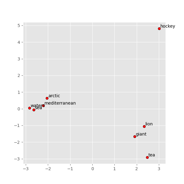
It’s important to note that this representation is learnt from the training dataset. That the training dataset matches our expectations is purely a result of the fact that the training dataset is a generic dataset. But if we were to choose a different, custom dataset, the embeddings can be expected to be placed differently on the graph.
LLM Model Embeddings
Word embeddings are great for human consumption, and then some more. But there are far too many words, and many words enter a language over time. Plus there are new Proper Nouns that get invented over time. And then, there are misspellings. Word embeddings miss out on these.
When looking to train more advanced networks using embeddings, we want our embeddings that capture further lower-level nuances of the language in question. Let’s take an example. Which of the following (currently non-existent in my knowledge) words are likely to be considered okay in a new piece of text you encounter?
- Zbwklttwq
- Queprayent
I’d guess you agree it’s Queprayent. Why? There’s something about our languages that makes us conclude so. We have no rules to explain, but one (of multiple) possible explanations is how the vowels make the word pronounceable and hence more palatable to us. With techniques like subword tokenization or byte-pair encoding, it’s possible to capture such nuances of a language.
When training LLMs, we could use the word embeddings. But if we trained our LLM with an embeddings model that captures further lower-level language nuances, we can hope to train networks better and also hope to get better outcomes for the various tasks we imagine using the LLMs for. That’s where using subword or byte-pair-encoded tokens come in.
LLM models have their own embeddings that are distinct from embeddings created from more human-understandable semantic entities like dictionary words. In other words, each LLM gets to decide its own embeddings model to train and use. When working with the model data, the embeddings model will be part of the distribution and only that can and will be used.
Let us look at an example embedding computed by meta-llama/Meta-Llama-3-8B
llama3_embeddings = load_embeddings(llama3_model_embeddings_extract_file)
llama3_tokenizer = AutoTokenizer.from_pretrained(llama3_model_name)

text_for_embeddings = "The oceans and the seas are filled with salty water, cried the earth."
# We need the return_tensors to be set to pt because the embeddings model expects a tensor in that format
text_tokens = llama3_tokenizer(text_for_embeddings, truncation=True, return_tensors="pt")
input_ids = text_tokens["input_ids"]

print(f"The input ids are: {input_ids}")
input_embeddings = llama3_embeddings(input_ids)
print("===== Embeddings =====")
print(input_embeddings)
Special tokens have been added in the vocabulary, make sure the associated word embeddings are fine-tuned or trained.
Asking to truncate to max_length but no maximum length is provided and the model has no predefined maximum length. Default to no truncation.
The input ids are: tensor([[  791, 54280,   323,   279, 52840,   527, 10409,   449, 74975,  3090,
            11, 39169,   279,  9578,    13]])
===== Embeddings =====
tensor([[[ 3.3760e-04, -3.0670e-03, -6.7139e-04,  ...,  7.0801e-03,
          -2.1057e-03,  2.6245e-03],
         [-1.1719e-02, -1.5259e-02,  1.9226e-03,  ...,  3.6469e-03,
           7.9346e-03, -9.8877e-03],
         [-5.5695e-04, -3.0365e-03,  8.2779e-04,  ...,  2.0313e-04,
           1.2589e-03,  5.0964e-03],
         ...,
         [ 7.1335e-04, -2.0294e-03, -1.2436e-03,  ...,  1.0910e-03,
          -5.7373e-03,  2.9297e-03],
         [ 6.6223e-03, -9.5215e-03, -5.0964e-03,  ...,  1.2741e-03,
           3.4790e-03,  3.8147e-03],
         [-8.7738e-04, -5.5313e-04, -1.4603e-05,  ...,  1.6403e-03,
           3.3951e-04,  1.7166e-03]]], grad_fn=<EmbeddingBackward0>)
To check the model architecture, let’s print out the structure of the meta-llama/Meta-Llama-3-8B model.
llama_model = AutoModel.from_pretrained(llama3_model_name)
print(llama_model)
Loading checkpoint shards:   0% 0/4 [00:00<?, ?it/s]
Loading checkpoint shards:  25% 1/4 [00:06<00:19,  6.61s/it]
Loading checkpoint shards:  50% 2/4 [00:19<00:20, 10.18s/it]
Loading checkpoint shards:  75% 3/4 [00:36<00:13, 13.40s/it]
Loading checkpoint shards: 100% 4/4 [00:36<00:00,  8.24s/it]
Loading checkpoint shards: 100% 4/4 [00:36<00:00,  9.21s/it]
LlamaModel(
  (embed_tokens): Embedding(128256, 4096)
  (layers): ModuleList(
    (0-31): 32 x LlamaDecoderLayer(
      (self_attn): LlamaSdpaAttention(
        (q_proj): Linear(in_features=4096, out_features=4096, bias=False)
        (k_proj): Linear(in_features=4096, out_features=1024, bias=False)
        (v_proj): Linear(in_features=4096, out_features=1024, bias=False)
        (o_proj): Linear(in_features=4096, out_features=4096, bias=False)
        (rotary_emb): LlamaRotaryEmbedding()
      )
      (mlp): LlamaMLP(
        (gate_proj): Linear(in_features=4096, out_features=14336, bias=False)
        (up_proj): Linear(in_features=4096, out_features=14336, bias=False)
        (down_proj): Linear(in_features=14336, out_features=4096, bias=False)
        (act_fn): SiLU()
      )
      (input_layernorm): LlamaRMSNorm()
      (post_attention_layernorm): LlamaRMSNorm()
    )
  )
  (norm): LlamaRMSNorm()
)
The embeddings layer is the first in sequence - its dimensions are \(128256 \times 4096\). Recall that the token vocabulary size of meta-llama/Meta-Llama-3-8B is 128256 and the embeddings dimension is 4096. The embeddings layer maps each token to a 4096 dimensional vector.
We don’t need to deal with the embeddings in LLMs directly, unlike GloVe. Both kinds of embeddings - those for LLMs, and those created from natural language words - serve different purposes.
Summing up…
Tokens and embeddings are the initial phases that any text encounters as it traverses through some network.
If you are looking to develop with, or build upon textual deep learning systems, understanding both of these is certainly a big advantage. Knowledge of tokenization and embeddings can also help you tune performance, and exploit better, systems like vector databases too. Vector databases work with embeddings, and they provide means to store documents and retrieve based on similarity scores. The similarity is defined by some distance measure in the vector-space of the embeddings. Knowing how a particular embedding model works will help you make better choices for your use-cases.
The next logical steps will be to explore how LLMs work - for our purposes - in code. If you liked this article so far, I hope you’ll like the following article too - which is in the works. Will link to it here when it’s ready.
References
- Let’s build GPT: from scratch, in code, spelled out.
- Inside the LLM: Visualizing the Embeddings Layer of Mistral-7B and Gemma-2B
- The code repository that goes along side the above video.
Supporting Code
The supporting code not found in the snippets above can be found below.
pyproject.toml
[tool.poetry]
name = "llm-for-the-experienced-beginner"
version = "0.1.0"
authors = ["Ravindra R. Jaju"]
description = "Supporting code for the article - Understanding Tokens and Embeddings with Code"

[tool.poetry.dependencies]
python = "^3.12"
scikit-learn = "^1.4.2"
transformers = "^4.39.3"
gensim = "^4.3.2"
numpy = "^1.26.4"
matplotlib = "^3.8.4"
torch = "^2.2.2"
huggingface-hub = "^0.22.2"
scipy = "<1.13"

[build-system]
requires = ["poetry-core"]
build-backend = "poetry.core.masonry.api"
Utils
import os
import torch
import torch.nn as nn
from functools import cache
from transformers import AutoTokenizer, AutoModel

class EmbeddingModel(nn.Module):
    def __init__(self, vocab_size, embedding_dim):
        super(EmbeddingModel, self).__init__()
        self.embedding = nn.Embedding(num_embeddings=vocab_size, embedding_dim=embedding_dim)

    def forward(self, input_ids):
        return self.embedding(input_ids)


def print_tokens(tokenizer, input_ids_tensor):
    token_texts = [tokenizer.decode([token_id], skip_special_tokens=True) for token_id in input_ids_tensor[0]]
    header = f"{'Token':<10} | {'ID':<8}"
    print(f"{'='*30}\n{'Tokens and their IDs':^30}\n{'='*30}")
    print(header)
    print(f"{'-'*10}-+-{'-'*17}")

    for idx, token_id in enumerate(input_ids_tensor[0]):
        token_text = token_texts[idx]
        print(f"{token_text:<10} | {token_id:<20}")

    print(f"{'='*30}")


def extract_embeddings(model_name, embeddings_filename, **kwargs):
    trust_remote_code = kwargs.pop("trust_remote_code", False)
    if not os.path.isfile(embeddings_filename):
        model = AutoModel.from_pretrained(model_name, trust_remote_code=trust_remote_code)
        embeddings = model.get_input_embeddings()
        print(f"Extracted embeddings layer for {model_name}: {embeddings}")
        torch.save(embeddings.state_dict(), embeddings_filename)
    else:
        print(f"File {embeddings_filename} already exists...")


# Optimizing on load times for REPL-workflows - we cache
@cache
def load_embeddings(embeddings_filename):
    embeddings_data = torch.load(embeddings_filename)
    weights = embeddings_data["weight"]
    vocab_size, dimensions = weights.size()

    embeddings = EmbeddingModel(vocab_size, dimensions)
    embeddings.embedding.weight.data = weights
    embeddings.eval()
    return embeddings
Code Files
Acknowledgements
In no specific order, I’d like to acknowledge specific and detailed feedback on the content and style from my colleagues
- Vinayak Kadam
- Rhushikesh Apte
- Sudarsan Balaji
- Preethi Srinivasan